感知机
感知机原理
感知机是一种二分类模型,其核心思想是:给定一个数据集,其中每个数据点都有一个特征向量,我们希望找到一个超平面,将数据分成两类,使得超平面尽可能多地分开两个类别的数据点。
感知机的学习目标是找到一个超平面,使得数据点到超平面的距离最大,即找到一个分割超平面,使得正负样本尽可能分开。
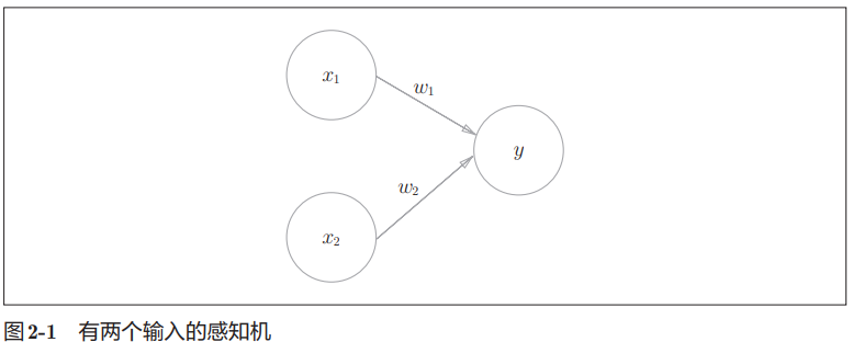
书中参考图是一个有两个输入信号 $x_1$ $x_2$ 的感知机。 $w_1$ 和 $w_2$ 是输入信号的权重(w 是 weight 的首字母)。 图中的大圆称为“神经元”或“节点”。 输入信号传入神经元时,会分别乘以固定的权重($x_{1}w_{1}$,$x_{2}w_{2}$),神经元会计算传送过来的信号的总和。 只有当这个总和超过了某个界限值时,才会输出 1。这也称为“神经元被激活”。这里将这个界限值称为阈值,用符号 θ 表示。
数学表达如下:
$$ y=\begin{cases} 0 & (w_1x_1 + w_2x_2 \le \theta) \ 1 & (w_1x_1 + w_2x_2 \gt \theta) \end{cases} $$
感知机的不同输入分别对应各自的权重,权重越大表示信号的重要性越高。
简单感知机构造
逻辑电路:与门/或门/与非门
以两个输入的感知机为例,我们可以构造逻辑电路与/或/与非门。
三种门逻辑电路对应上图两个输入的感知机模型,假设输入信号取值范围是 0 或 1,实现逻辑门的权重和 $\theta$ 取值表如下。
| gate | $w_1$ | $w_2$ | $\theta$ |
|---|---|---|---|
| and | 1.0 | 1.0 | $(1, 2)$ |
| or | 1.0 | 1.0 | $(0, 1)$ |
| not and | -1.0 | -1.0 | $(-2, -1)$ |
python 实现如下。
import numpy as np


class Perceptron:
    """
    感知机模型
    """

    def __init__(self, weights: np.ndarray):
        self.weights = weights

    def evaluate(self, x: np.ndarray) -> bool:
        return (x*self.weights).sum()


print('与门感知机,权重 [1. 1.] theta 取值区间 (1,2)')
p_and = Perceptron(np.array([1., 1.]))

p_theta = 1.1
x = np.array([0., 0.])
y = p_and.evaluate(x)
print(f'x={x}, theta={p_theta}, result =', y, 'activated ', y > p_theta)
x = np.array([1., 0.])
y = p_and.evaluate(x)
print(f'x={x}, theta={p_theta}, result =', y, 'activated ', y > p_theta)
x = np.array([0., 1.])
y = p_and.evaluate(x)
print(f'x={x}, theta={p_theta}, result =', y, 'activated ', y > p_theta)
x = np.array([1., 1.])
y = p_and.evaluate(x)
print(f'x={x}, theta={p_theta}, result =', y, 'activated ', y > p_theta)
与门感知机,权重 [1. 1.] theta 取值区间 (1,2)
x=[0. 0.], theta=1.1, result = 0.0 activated  False
x=[1. 0.], theta=1.1, result = 1.0 activated  False
x=[0. 1.], theta=1.1, result = 1.0 activated  False
x=[1. 1.], theta=1.1, result = 2.0 activated  True
偏置和 theta
如果说权重表示输入的重要程度,偏置项(bias)就表示神经元被激活的容易程度。按感知机的定义,偏置项越高,则神经元越容易激活。
将偏置项 $b$ 定义为 $-\theta$ 则有下面的感知机模型。
$$ y=\begin{cases} 0 & (w_1x_1 + w_2x_2 + b \le 0) \ 1 & (w_1x_1 + w_2x_2 + b \gt 0) \end{cases} $$
可以看成 $\theta$ 为$0$的感知机模型,同时增加了一个偏置项。
python 定义如下。
class Perceptron:
    """
    感知机模型
    """

    def __init__(self, weights: np.ndarray, bias: float):
        self.weights = weights
        self.bias = bias

    def evaluate(self, x: np.ndarray) -> bool:
        return np.sum(x*self.weights)+self.bias > 0
感知机的局限
这里需要一点高中数学知识。
以与门感知机为例,简化起见,权重设为 1,偏置设为-2.0,将权重和偏置代入感知机定义公式。
$$ y=\begin{cases} 0 & (x_1 + x_2 - 2.0 \le 0) \ 1 & (x_1 + x_2 - 2.0 \gt 0) \end{cases} $$
把不等式方程组画出图像,会发现是一个被 $x_1 + x_2 - 2.0 = 0$ 这条直线分割的两块空间。一块空间表示真值一块表示假。
import numpy as np
import matplotlib.pyplot as plt

x1 = np.arange(-3, 3, 0.1)
x2 = 2.0-x1

plt.plot([0, 2], [2, 0], 'go', markersize=5)
plt.fill([-3, -3, 3, -3], [5, -1, -1, 5], 'red', alpha=0.5)
plt.plot(x1, x2)
plt.axhline(y=0, color='k')
plt.axvline(x=0, color='k')
plt.grid(True, axis='both',linestyle=':')
plt.show()
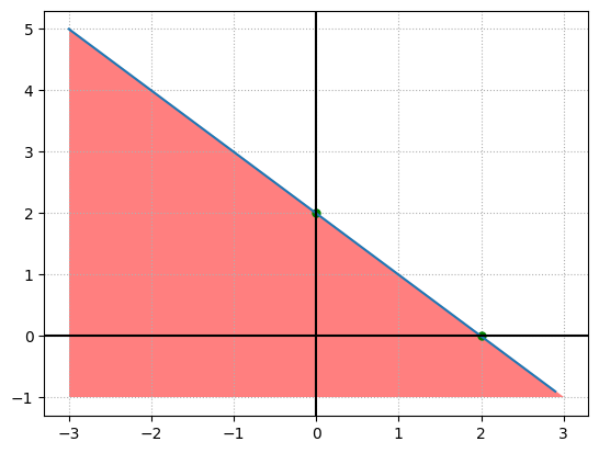
可以直观地看到,当输入的 $x_1$、$x_2$ 构成的点落在图中红色区域内,感知机输出假。反之输出真。
以与门为例。
import numpy as np
import matplotlib.pyplot as plt

x1 = np.arange(-3, 3, 0.1)
x2 = 1.1-x1

plt.plot(x1, x2)
plt.plot(
    np.array([0., 0., 1., 1.]),
    np.array([1., 0., 1., 0.]),
    'go')
plt.axhline(y=0, color='k')
plt.axvline(x=0, color='k')
plt.grid(True, axis='both', linestyle=':')
plt.show()
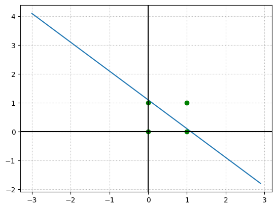
当图中 $1<\theta<2$ 且有 $x_1=1,x_2=1$,蓝色点才会落到白色区域。而直线上的点按我们的感知机定义,会视为假值。
当我们修改偏置值时,这条直线就会上下移动。
- 当 $1<\theta<2$ 时,感知机就变成了与逻辑门,(1,1)被视为真值,(1,0)和(0,1)都被视为假值。
- 当 $0<\theta<1$ 时,则感知机就变成了或逻辑门,(1,0)和(0,1)都被视为真值。
- 当 $-2<\theta< -1$ 时且权值 $w_1=-1,w_2=-1$,图形中红色区域和白色区域反转,(0,0),(0,1),(1,0) 视为真值,直线位置和 $1<\theta<2$ 范围一致。
当需要分类的输入组合是 (0,0),(1,1) 和 (1,0),(0,1) 时,感知机就无法正确分类了。
对于这种情况,可以引入多层感知机。
多层感知机
多层感知机就是多个感知机的堆叠。
读过数电应该知道区分 (0,0)(1,1) 和 (1,0)(0,1) 其实就是实现一个异或门,不同时输出 1,相同时输出 0。
而异或门本身可以由或门、与非门和与门组成。
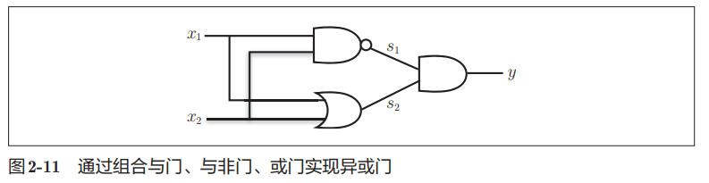
这里用 python 构建出多层感知机。
class Perceptron:
    """
    感知机模型
    """

    def __init__(self, weights: np.ndarray, bias: float):
        self.weights = weights
        self.bias = bias

    def evaluate(self, x: np.ndarray) -> bool:
        return np.sum(x*self.weights)+self.bias > 0


def xor(x1: float, x2: float) -> bool:
    p_nand = Perceptron(np.array([-1.0, -1.0]), 1.5)
    p_or = Perceptron(np.array([1.0, 1.0]), -0.5)
    p_and = Perceptron(np.array([1.0, 1.0]), -1.5)

    s1 = 1.0 if p_nand.evaluate(np.array([x1, x2])) else 0.0
    s2 = 1.0 if p_or.evaluate(np.array([x1, x2])) else 0.0
    return p_and.evaluate(np.array([s1, s2]))


print('xor(0.0, 0.0)=', xor(0.0, 0.0))
print('xor(0.0, 1.0)=', xor(0.0, 1.0))
print('xor(1.0, 0.0)=', xor(1.0, 0.0))
print('xor(1.0, 1.0)=', xor(1.0, 1.0))
xor(0.0, 0.0)= False
xor(0.0, 1.0)= True
xor(1.0, 0.0)= True
xor(1.0, 1.0)= False
尾声
读完这一章有几个疑问:
- 多层感知机能表示表示非线性空间,能给多层感知机画出函数图像吗?长什么样?
- 如果给两个样本集合,怎么判断这个两个集合能不能被单层感知机分类?